一、聚类简介

1、概述

        实质上是机器学习中的一种无监督学习方法。并不需要我们对数据进行标记。通常，它被用作在一组示例中找到有意义的结构、解释性基础过程、生成特征、进行分组的等。

        聚类是将总体或数据点划分为多个组的任务，以使同一组中的数据点与同一组中的其他数据点更相近。

         例如下面的分簇

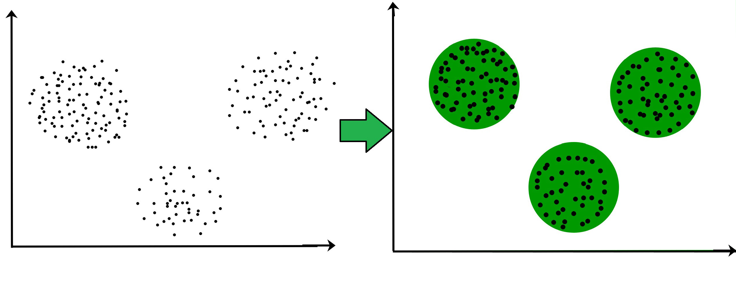
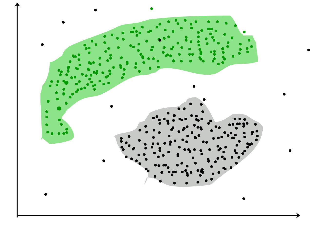
但是簇不总是规则形状的。

2、常见应用 

        在癌细胞的识别中：聚类算法被广泛用于癌细胞的识别。它将癌性和非癌性数据集分为不同的组。

        在搜索引擎中：搜索引擎也适用于集群技术。搜索结果基于最接近搜索查询的对象显示。它通过将相似的数据对象分组到远离其他不同对象的一组中来实现。查询的准确结果取决于所使用的聚类算法的质量。

        客户细分：它用于市场研究，根据客户的选择和偏好对客户进行细分。

        在生物学中：它在生物学流中使用图像识别技术对不同种类的植物和动物进行分类。

        在土地利用方面：聚类技术用于识别 GIS 数据库中类似土地利用的区域。这对于发现特定土地应该用于什么目的，这意味着它更适合哪种目的非常有用。

二、聚类算法的思想

        聚类算法有多种类型。已知发布的可能超过了近百种算法。我们先了解最常见的一些算法。

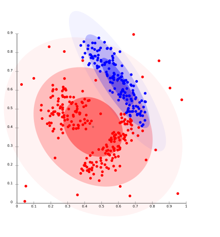
1、基于分布的算法

        基于分布的聚类生成的聚类假定数据背后有明确定义的数学模型，这对于某些数据分布来说是一个比较生硬的假设。 分组是通过假设一些分布通常为Gaussian Distribution来完成的。例如，使用高斯混合模型 (GMM)的期望最大化聚类算法的典型示例。

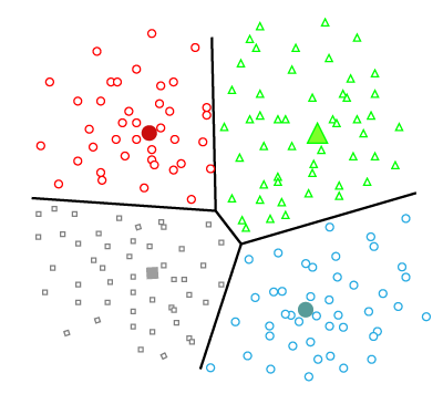
2、基于质心的算法

        也被称为分区聚类，这基本上是一种迭代聚类算法，其中通过数据点与聚类质心的接近程度形成聚类。这里，形成聚类中心，即质心，使得数据点与中心的距离最小。这个问题基本上是 NP-Hard 问题之一，因此解决方案通常会在多次试验中得到近似。 

         K–means算法是该算法的典型示例。这个算法最大的问题是我们需要提前指定 K。

3、基于连通性的算法

        连通性的模型的核心思想类似于基于质心的模型，它基本上是根据数据点的接近程度来定义集群。在这里，我们研究了一个概念，即更近的数据点与更远的数据点具有相似的行为。 
它不是数据集的单一分区，而是提供了广泛的集群层次结构，这些集群在一定距离处相互合并。这里距离函数的选择是主观的。这些模型很容易解释，但缺乏可扩展性。 

4、基于密度的算法

        在此聚类模型中，将在数据空间中搜索数据空间中数据点密度不同的区域。它根据数据空间中存在的不同密度隔离各种密度区域。 

        典型的算法，比如DBSCAN和OPTICS。 

5、基于层次的算法

        该方法中形成的簇形成基于层次的树型结构。使用先前形成的集群形成新的集群。它分为两类。

        凝聚式（自下而上的方法），自下而上的方法在低维空间中找到密集区域，然后组合形成集群。

        分裂（自上而下的方法），自上而下的算法在完整的维度集中找到一个初始聚类并评估每个聚类的子空间。

        这种方法最常见的例子是Agglomerative Hierarchical算法。

6、模糊聚类

        模糊聚类是一种软方法，其中数据对象可能属于多个组或集群。每个数据集都有一组隶属系数，这些系数取决于在集群中的隶属程度。Fuzzy C-means算法就是这种聚类的例子；它有时也称为模糊 k 均值算法。

三、最流行的聚类算法

        K-Means 算法： k-means 算法是最流行的聚类算法之一。它通过将样本分成等方差的不同集群来对数据集进行分类。必须在此算法中指定集群的数量。它速度很快，所需的计算量更少，线性复杂度为O(n)。

        Mini-Batch K-Means算法：Mini-Batch K-Means 是 k-means 的修改版本，它使用小批量样本而不是整个数据集来更新集群质心，这可以使其更快地处理大型数据集，并且可能对统计噪声更稳健。

        Mean-shift算法： Mean-shift算法试图在数据点的平滑密度中找到密集区域。这是一个基于质心的模型的示例，它致力于将质心的候选者更新为给定区域内点的中心。

        DBSCAN 算法：它代表具有噪声的应用程序的基于密度的空间聚类。它是类似于均值偏移的基于密度的模型的示例，但具有一些显着的优势。在该算法中，高密度区域被低密度区域隔开。因此，可以找到任意形状的簇。

        OPTICS算法：这种聚类技术不同于其他聚类技术，因为这种技术没有明确地将数据分割成簇。相反，它会生成可达距离的可视化，并使用此可视化对数据进行聚类。

        Spectral Clustering：一种基于于图论的技术，该方法用于根据连接节点的边来识别图中节点的社区。

        高斯混合模型（Mixture of Gaussians）：该算法可用作 k-means 算法或 K-means 可能失败的情况的替代方案。在 GMM 中，是需要假设数据点是高斯分布的。

        凝聚层次算法（Agglomerative Clustering）：凝聚层次算法执行自下而上的层次聚类。在这种情况下，每个数据点一开始就被视为一个集群，然后依次合并。集群层次结构可以表示为树结构。

        Affinity Propagation：它与其他聚类算法不同，因为它不需要指定聚类的数量。在这种情况下，每个数据点在这对数据点之间发送一条消息，直到收敛。它具有 O(N 2 T) 时间复杂度，这是该算法的主要缺点。

        BIRCH：BIRCH 聚类（BIRCH 是 Balanced Iterative Reducing and Clustering using
Hierarchies 的缩写）涉及构建一个树形结构，从中提取聚类质心。BIRCH 增量和动态地对传入的多维度量数据点进行聚类，以尝试使用可用资源（即可用内存和时间限制）产生最佳质量的聚类。

四、示例

1、生成数据集

        我们使用make_classification() 函数来创建一个测试二分类数据集，并应用上面的聚类算法查看效果。

X, y = make_classification(n_samples=1000, n_features=2, n_informative=2, n_redundant=0, n_clusters_per_class=1, random_state=4)# create scatter plot for samples from each classfor class_value in range(2):# get row indexes for samples with this classrow_ix = where(y == class_value)# create scatter of these samplespyplot.scatter(X[row_ix, 0], X[row_ix, 1])# show the plotpyplot.show()

         数据可视化

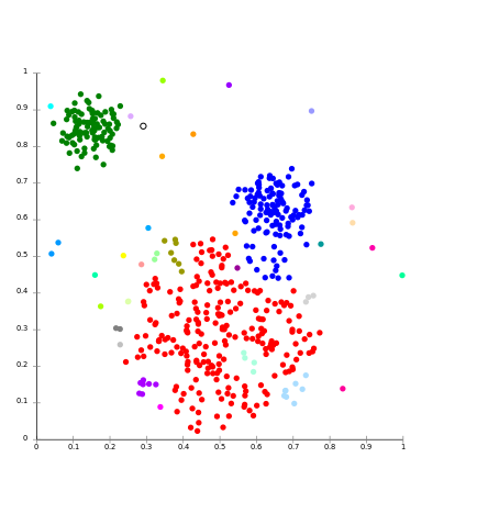
 2、Affinity Propagation

         参考代码

from numpy import uniquefrom numpy import wherefrom sklearn.datasets import make_classificationfrom sklearn.cluster import AffinityPropagationfrom matplotlib import pyplot# define datasetX, _ = make_classification(n_samples=1000, n_features=2, n_informative=2, n_redundant=0, n_clusters_per_class=1, random_state=4)# define the modelmodel = AffinityPropagation(damping=0.9)# fit the modelmodel.fit(X)# assign a cluster to each exampleyhat = model.predict(X)# retrieve unique clustersclusters = unique(yhat)# create scatter plot for samples from each clusterfor cluster in clusters:# get row indexes for samples with this clusterrow_ix = where(yhat == cluster)# create scatter of these samplespyplot.scatter(X[row_ix, 0], X[row_ix, 1])# show the plotpyplot.show()

        可视化结果，结果不是很理想。

 3、Agglomerative Clustering

        参考代码

# agglomerative clusteringfrom numpy import uniquefrom numpy import wherefrom sklearn.datasets import make_classificationfrom sklearn.cluster import AgglomerativeClusteringfrom matplotlib import pyplot# define datasetX, _ = make_classification(n_samples=1000, n_features=2, n_informative=2, n_redundant=0, n_clusters_per_class=1, random_state=4)# define the modelmodel = AgglomerativeClustering(n_clusters=2)# fit model and predict clustersyhat = model.fit_predict(X)# retrieve unique clustersclusters = unique(yhat)# create scatter plot for samples from each clusterfor cluster in clusters:# get row indexes for samples with this clusterrow_ix = where(yhat == cluster)# create scatter of these samplespyplot.scatter(X[row_ix, 0], X[row_ix, 1])# show the plotpyplot.show()

        可视化结果，还算找到了一个偏差不是特别大的结果。 

4、BIRCH

        参考代码

from numpy import uniquefrom numpy import wherefrom sklearn.datasets import make_classificationfrom sklearn.cluster import Birchfrom matplotlib import pyplot# define datasetX, _ = make_classification(n_samples=1000, n_features=2, n_informative=2, n_redundant=0, n_clusters_per_class=1, random_state=4)# define the modelmodel = Birch(threshold=0.01, n_clusters=2)# fit the modelmodel.fit(X)# assign a cluster to each exampleyhat = model.predict(X)# retrieve unique clustersclusters = unique(yhat)# create scatter plot for samples from each clusterfor cluster in clusters:# get row indexes for samples with this clusterrow_ix = where(yhat == cluster)# create scatter of these samplespyplot.scatter(X[row_ix, 0], X[row_ix, 1])# show the plotpyplot.show()

        可视化结果，找到了一个很好的分组。 

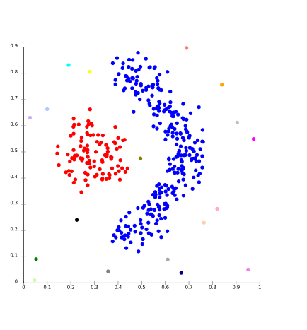
 5、DBSCAN

        参考代码

# dbscan clusteringfrom numpy import uniquefrom numpy import wherefrom sklearn.datasets import make_classificationfrom sklearn.cluster import DBSCANfrom matplotlib import pyplot# define datasetX, _ = make_classification(n_samples=1000, n_features=2, n_informative=2, n_redundant=0, n_clusters_per_class=1, random_state=4)# define the modelmodel = DBSCAN(eps=0.30, min_samples=9)# fit model and predict clustersyhat = model.fit_predict(X)# retrieve unique clustersclusters = unique(yhat)# create scatter plot for samples from each clusterfor cluster in clusters:# get row indexes for samples with this clusterrow_ix = where(yhat == cluster)# create scatter of these samplespyplot.scatter(X[row_ix, 0], X[row_ix, 1])# show the plotpyplot.show()

        可视化结果，结果还是比较不错的。

6、K-Means

        参考代码

# k-means clusteringfrom numpy import uniquefrom numpy import wherefrom sklearn.datasets import make_classificationfrom sklearn.cluster import KMeansfrom matplotlib import pyplot# define datasetX, _ = make_classification(n_samples=1000, n_features=2, n_informative=2, n_redundant=0, n_clusters_per_class=1, random_state=4)# define the modelmodel = KMeans(n_clusters=2)# fit the modelmodel.fit(X)# assign a cluster to each exampleyhat = model.predict(X)# retrieve unique clustersclusters = unique(yhat)# create scatter plot for samples from each clusterfor cluster in clusters:# get row indexes for samples with this clusterrow_ix = where(yhat == cluster)# create scatter of these samplespyplot.scatter(X[row_ix, 0], X[row_ix, 1])# show the plotpyplot.show()

        可视化结果， 找到了一个合理的分组（尽管不适合这个数据集，但是从可视化的结果来看是找到了两个还算合理的簇，所以说是一个合理的分组）。

7、Mini-Batch K-Means

        参考代码

from numpy import uniquefrom numpy import wherefrom sklearn.datasets import make_classificationfrom sklearn.cluster import MiniBatchKMeansfrom matplotlib import pyplot# define datasetX, _ = make_classification(n_samples=1000, n_features=2, n_informative=2, n_redundant=0, n_clusters_per_class=1, random_state=4)# define the modelmodel = MiniBatchKMeans(n_clusters=2)# fit the modelmodel.fit(X)# assign a cluster to each exampleyhat = model.predict(X)# retrieve unique clustersclusters = unique(yhat)# create scatter plot for samples from each clusterfor cluster in clusters:# get row indexes for samples with this clusterrow_ix = where(yhat == cluster)# create scatter of these samplespyplot.scatter(X[row_ix, 0], X[row_ix, 1])# show the plotpyplot.show()

        可视化结果，和k-means结果十分接近。

 8、Mean Shift

        参考代码

# mean shift clusteringfrom numpy import uniquefrom numpy import wherefrom sklearn.datasets import make_classificationfrom sklearn.cluster import MeanShiftfrom matplotlib import pyplot# define datasetX, _ = make_classification(n_samples=1000, n_features=2, n_informative=2, n_redundant=0, n_clusters_per_class=1, random_state=4)# define the modelmodel = MeanShift()# fit model and predict clustersyhat = model.fit_predict(X)# retrieve unique clustersclusters = unique(yhat)# create scatter plot for samples from each clusterfor cluster in clusters:# get row indexes for samples with this clusterrow_ix = where(yhat == cluster)# create scatter of these samplespyplot.scatter(X[row_ix, 0], X[row_ix, 1])# show the plotpyplot.show()

        可视化结果

 9、OPTICS

        参考代码

from numpy import uniquefrom numpy import wherefrom sklearn.datasets import make_classificationfrom sklearn.cluster import OPTICSfrom matplotlib import pyplot# define datasetX, _ = make_classification(n_samples=1000, n_features=2, n_informative=2, n_redundant=0, n_clusters_per_class=1, random_state=4)# define the modelmodel = OPTICS(eps=0.8, min_samples=10)# fit model and predict clustersyhat = model.fit_predict(X)# retrieve unique clustersclusters = unique(yhat)# create scatter plot for samples from each clusterfor cluster in clusters:# get row indexes for samples with this clusterrow_ix = where(yhat == cluster)# create scatter of these samplespyplot.scatter(X[row_ix, 0], X[row_ix, 1])# show the plotpyplot.show()

        可视化结果，没有得到相对合理的结果，不太适合这个数据集。

 10、Spectral Clustering

        参考代码

from numpy import uniquefrom numpy import wherefrom sklearn.datasets import make_classificationfrom sklearn.cluster import SpectralClusteringfrom matplotlib import pyplot# define datasetX, _ = make_classification(n_samples=1000, n_features=2, n_informative=2, n_redundant=0, n_clusters_per_class=1, random_state=4)# define the modelmodel = SpectralClustering(n_clusters=2)# fit model and predict clustersyhat = model.fit_predict(X)# retrieve unique clustersclusters = unique(yhat)# create scatter plot for samples from each clusterfor cluster in clusters:# get row indexes for samples with this clusterrow_ix = where(yhat == cluster)# create scatter of these samplespyplot.scatter(X[row_ix, 0], X[row_ix, 1])# show the plotpyplot.show()

        可视化结果

 11、Gaussian Mixture Model

        参考代码

# gaussian mixture clusteringfrom numpy import uniquefrom numpy import wherefrom sklearn.datasets import make_classificationfrom sklearn.mixture import GaussianMixturefrom matplotlib import pyplot# define datasetX, _ = make_classification(n_samples=1000, n_features=2, n_informative=2, n_redundant=0, n_clusters_per_class=1, random_state=4)# define the modelmodel = GaussianMixture(n_components=2)# fit the modelmodel.fit(X)# assign a cluster to each exampleyhat = model.predict(X)# retrieve unique clustersclusters = unique(yhat)# create scatter plot for samples from each clusterfor cluster in clusters:# get row indexes for samples with this clusterrow_ix = where(yhat == cluster)# create scatter of these samplespyplot.scatter(X[row_ix, 0], X[row_ix, 1])# show the plotpyplot.show()

        可视化结果，十分完美，因为数据集是由高斯混合生成的。